What is Entropy?

Entropy is a central quantity in many different fields, and accordingly there are a bunch of "derivations" to arrive at the same formula. At the very basic level, entropy is commonly used to mean the "uncertainty" or "disorder" of a system.

Entropy via Physics

But what does that actually mean? On one hand we can take the physics route. In stat mech, we have the idea of a "microstates," which define the particular configuration of particles in a system, and these configurations give rise to "macrostates," which is what we can observe. In general, a macrostate consists of many microstates. So for example, a system may be defined by $N$ particles, each with some sort of 3D momentum, spin, etc. The particular configuration of those $N$ particles would be the microstate, but macrostates of the system would be something like energy, pressure, number of particles, etc. So many microstates can correspond to the same macrostate: if our macrostate is the system at a particular energy $E$, many microstates (ie. particular configurations of the $N$ particles) correspond to the same total energy $E$.

Suppose we fix a macrostate, that is we fix the system to be at energy $E$ with generalized coordinates $\textbf{x}$ (taking from Kardar's language). The central postulate of stat mech is that given this conditioning, all valid microstates are equally likely. That is, our distribution over microstates is

where $\mathcal{H}$ represents the Hamiltonian. We want some sort of function $S(\Omega)$ which describes how much "uncertainty" over microstates this particular macrostate has. What sort of properties should this function have?

• If two systems with $\Omega_1$ and $\Omega_2$ microstates are independent, the combined system has $\Omega_1 \Omega_2$ microstates (this just follows from counting), so we want $S(\Omega_1 \Omega_2) = S(\Omega_1) + S(\Omega_2)$ -- entropy should be "extensive" (additive over independent systems). This requirement is a bit hand-wavy but given "phenomologically" by classical thermodynamics. I'm not fully convinced I understand the additivity requirement, and any "derivation" I see online starts with the fact that entropy is log-based, which puts the cart before the horse.
• $S$ should be monotonically increasing in $\Omega$: more microstates means more uncertainty. I can get by this!
• $S(1) = 0$: a system with only one possible microstate has no uncertainty. This also makes sense!

These three properties uniquely determine $S$ up to a constant. The functional equation $S(mn) = S(m) + S(n)$ on positive integers, combined with monotonicity, forces $S(\Omega) = c \log \Omega$ for some $c > 0$ (cauchy's log equation). And in physics, the constant that makes the units work out is $k_B$, Boltzmann's constant, giving

Setting $k_B = 1$, this says entropy is the log-number of accessible microstates -- or equivalently, how many bits you'd need to specify the system's microstate. Alternatively, it's also the entropy of a uniform probability distribution over a state space of size $|\Omega|$, going back to our central postulate of stat mech that all microstates for a particular macrostate are equally likely.

Entropy via Information Theory

The above derivation holds for the specific case of the uniform microcanonical distribution, but what we really want is some measure of uncertainty over general probability distributions. This sort of thing lies outside the purview of physics (as wonderful as it is) and leads us to the info theory derivation of entropy. Specifically, the Shannon-Kinchin theorem derives the entropy formula from a few guiding principles (similar to above): given any distribution $p = (p_1, \ldots, p_n)$ over $n$ outcomes, we want a function $H(p_1, \ldots, p_n)$ satisfying:

1. Continuity: $H$ is continuous in all $p_i$.
2. Maximality: $H(p_1, \ldots, p_n) \leq H(1/n, \ldots, 1/n)$ -- uniform has maximum entropy.
3. Expandability: $H(p_1, \ldots, p_n, 0) = H(p_1, \ldots, p_n)$ -- adding an impossible outcome doesn't change entropy.
4. Chain rule: Entropy decomposes over groupings:

WE usually learn the chain rule as a side effect of the entropy formula, but I guess it's one of the axioms under which it's built.

Theorem (Shannon-Khinchin): The only functions satisfying these four axioms are

for some $\lambda > 0$.

Proof sketch. First consider the uniform case $H_n = H(1/n, \ldots, 1/n)$, which is what we did in the stat mech microcanonical ensemble example. Applying the chain rule, a uniform distribution over $mn$ outcomes decomposes into choosing one of $m$ equal blocks, then one of $n$ outcomes within the block -- both uniform -- so

This is the same equation we saw above, which with continuity it forces $H_n = \lambda \log n$.

For a non-uniform distribution with rational $p_i = k_i/N$ (where $\sum k_i = N$), we can think of it as a uniform distribution over $N$ outcomes grouped into blocks of sizes $k_1, \ldots, k_n$. The chain rule gives

(the $\lambda \log N$ on the left is $H_N$ the uniform distribution entropy, and the rhs is the expected within-block entropy).Then rearranging gives

Continuity extends this to all reals.

Note this recovers the physics formula: in the microcanonical ensemble $p_i = 1/\Omega$ for all $i$, so $H = -\sum_{i=1}^\Omega \frac{1}{\Omega}\log\frac{1}{\Omega} = \log \Omega$. The starting axioms are also very similar in flavor.

What is Entropy, Really?

The last place I expected to see entropy resurface was in our stat 205b (Berkeley probability theory class) unit on ergodic theory (to be fair, I had no prior knowledge of ergodic theory, so I guess I couldn't really expect anything). Broadly speaking, ergodic theory deals with "long-term behavior of dynamical systems."

When we say dynamical systems, the easiest way to think of it is as some space (say a set $S$) that undergoes a transformation (ie. "dynamics") every timestep, which can be given by some map $T : S \to S$. We care about how our initial space $S$ "evolves" as we keep applying $T$. This idea gives rise to the notion of "orbits." For a particular point $x \in S$, we can define its orbit as $\{T^n x : n \in \mathbb{N}\}$. If we think of this as a physical system with $x$ as some initial position, this orbit describes what kind of "path" over the space this point will trace out as we keep applying our dynamics. Metric entropy then arises as a notion of "orbit complexity" for a particular map $T$. This is all sounding too general, so lets formalize everything.

Ergodic Theory

The first phenomenon that's of interest is the idea of recurrence: if we take a set $E$, what can we say about the behavior of the orbits of points $x \in E$? For a particular type of map (measure preserving), we have the following result:

Definition: Poincare Recurrence: If $T$ is measure preserving and and $E$ is measurable, for almost every $x \in E$, there are infinitely many $n$ such that $T^n x \in E$.

I tried to draw this out until I realized the all-powerful Claude can just generate a much better looking diagram:

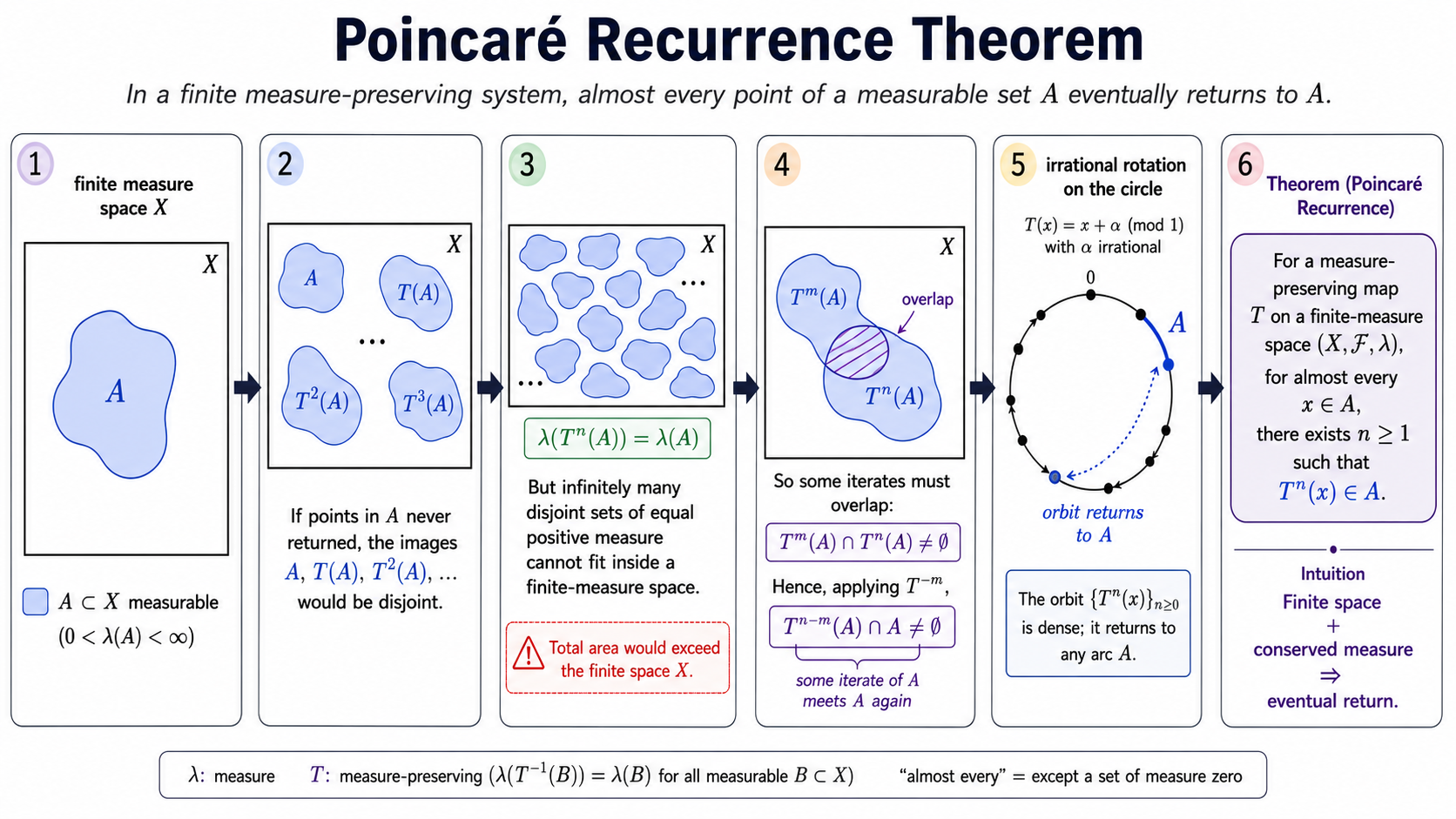
Ergodicity then gives an idea of "indecomposability" of sorts for invariant sets -- a system is ergodic if for any $B \in \mathcal{B}$ for a measure preserving $T$, all invariant sets (ie. $T^{-1}(B) = B$) must be measure zero or one. In this sense, we cannot take an invariant subset and "decompose" it further into smaller sets.

The whole point of talking about ergodic theory in this writeup is to see how the idea of entropy evolves as a natural measure of "orbit complexity" -- that is, for different ergodic systems, we'll see a difference in roughly speaking how "complex" the orbits generated by these systems are.

First, it's helpful to look at a couple of examples of ergodic systems:

Example 1: The Bernoulli Shift

Let $\Omega = \{0, 1\}^{\mathbb{Z}}$ with the product measure

and let $T$ be the left shift: $(T\omega)_n = \omega_{n+1}$. This is basically the canonical model for an i.i.d. coin-flip sequence, and $T$ just slides our view of the sequence one step forward.

Why is this ergodic? Suppose $A$ is a $T$-invariant set, so $T^{-1}A = A$. Because the sequence is invariant under the shift, membership in $A$ can only depend on the "tail" of the sequence. By Kolmogorov's 0-1 law, any tail event has probability 0 or 1 -- so $\mu_p(A) \in \{0, 1\}$.

Example 2: The Irrational Rotation

Let $\mathbb{T} = \mathbb{R}/\mathbb{Z}$ (the circle), with Lebesgue measure $\lambda$, and fix $\alpha \in \mathbb{R} \setminus \mathbb{Q}$. Define

Unlike the last example which has some stochasticity in the Bernoulli measure choice per point, here the map is completely deterministic and simply just rotations around the circle.

Proof of ergodicity: This is a bit more involved. We start with proving a useful intermediate formula, namely that there is some interval $I$ such that for small $\epsilon > 0$,

that is, $A$ intersects with at least $1-\epsilon$ fraction of this interval.

Subproof: A useful tool here is the inner regularity of Lebesgue measure: that is, any measurable $A$ satisfies $\lambda(A) = \sup\{\lambda(F) : F \subseteq A, F \text{ compact and measurable }\}$.

So inner regularity gives us some $K \subset A, \lambda(K) > 0$. Likewise by outer regularity we can get an open set $U$ where $\lambda(K) > \lambda(U) (1 - \epsilon)$ (choose a big enough $K$ and small enough $U$ where $K \subset A \subset U$). But the subset identity implies that $A \cap U \supset K$ so it follows that

And every open set $U$ on $\mathbb{T}$ can be expressed as disjoint subset of intervals $\sqcup_{j = 1}^\infty I_j$, so $\lambda(A \cap U) = \sum_{j} \lambda(A \cap I_j)$. At least one $I_j$ must satisfy the original identity by $U$ (else sum them and $U$ won't satisfy the original inequality, a contradiction). This completes the subproof.

Return to main proof: Now with this interval $I$, take the orbit $\{n \alpha \mod 1 : n \in \mathbb{Z}\}$, which is dense in $\mathbb{T}$. By density, now select $0 < n_0 < n_1 < \cdots < n_k$ so $I_j \triangleq I + n_j \alpha$ (mod 1) cover the whole circle up to some $\delta > 0$.

Because $A$ is invariant under $T$, it occupies at least $(1-\epsilon)$ fraction of $I_j$. For $T_\alpha^{n_j} (A) = A$, and $T_\alpha$ is measure preserving, so

and likewise $\lambda(I_j) = \lambda(I)$ and so the same inequality holds for any iterate $I_j$ of $I$. If $A$ covers at least $(1-\epsilon)$ of all the $I_j$, then it must cover at least $(1-\epsilon)$ of their union, but their union was chosen such that they cover at least measure $(1-\delta)$, and so $\lambda(A) \geq (1 - \epsilon)(1-\delta)$. Both variables were chosen arbitrarily, so it follows that $\lambda(A) = 1$.

So both of these systems are ergodic, but have very different "structure": in the first example, it is the tail behavior of probabilistic events that provide ergodicity. But in the above case, it is instead this "uniformity" of orbits across the circle that bring ergodicity.

Comparing Orbit Complexity

Seeing both of the previous systems suggests the idea that perhaps there should be a way to quantify how "complex" a system's orbits are. With this goal in mind, we can try and come up with ways to formalize this idea. One intuition we might have is that a more "complex" system should somehow generate a much more diverse set of orbits that all look different from one another. From an info theory perspective (which is sort've cheating by already knowing the end result), the idea of a "typical set" might be useful here, in particular what is the size (or number of orbits) that comprise a certain amount of probability space.

To formalize this idea, we will think of the "diversity of space that each orbit traverses through." Suppose we take a partition $\mathcal{P} = \{P_1, \ldots, P_k\}$ of $X$, then we can encode the orbit of any point $x$ as a symbolic sequence: record which partition element the orbit visits at each time step. For time $0$ through $N-1$, we get a word of length $N$:

Now a clear definition of complexity arises from this, namely the number of distinct words of length $N$ that would show up from orbits. We can take our two systems from before as case studies:

Bernoulli shift: We can do our partition $\mathcal{P}$ based on the 0th coordinate (so $P_0 = \{\omega_0 = 0\}$ points and $P_1 = \{\omega_0 = 1\}$ points). Then $\mathcal{P}_N(\omega) = (\omega_0, \ldots, \omega_{N-1})$, just a binary string of length $N$.

By the law of large numbers, most of the measure is on sequences with about $pN$ ones.Specifically, if we take $S_N(\omega) = \sum_{i = 0}^{N-1} \omega_i$, then LLN gives us that $\frac{S_N(\omega)}{N} \to p$ almost surely (each $\omega_i$ is sampled iid from Bernoulli(p)), meaning it also converges in measure.

The total measure carried by blocks $k \approx pN$ (reminiscent of typical set in info theory) is

Then, Stirling's approximation gives that the number of such sequences is roughly $\binom{N}{pN} \approx e^{N H(p)}$, where

is the binary entropy. Each individual typical sequence has measure $\approx e^{-N H(p)}$, so you need roughly $e^{N H(p)}$ of them to account for a fixed fraction of the total measure. What we see here is that the number of distinct length-$N$ blocks grows exponentially with $N$.

Irrational rotation: Fix a partition into $k$ intervals $\{I_1, \ldots, I_k\}$. The word $(j_0, \ldots, j_{N-1})$ occurs for initial point $x$ iff $x + n\alpha \in I_{j_n}$ for each $n$, meaning $x$ sits in the intersection $\bigcap_n (I_{j_n} - n\alpha)$. Each such intersection is an interval (or empty), and the endpoints of all these intervals come from at most $kN$ points on $\mathbb{T}$. So there are at most $kN$ distinct words of length $N$. For $k=2$ this is at most $N+1$. So here, the number of distinct orbit words only grows linearly in $N$.

So even though both systems are ergodic (time averages = space averages), the Bernoulli shift generates exponentially many distinguishable orbit patterns, while the rotation generates barely any. This is the qualitative picture of "orbit complexity."

Note on Initial Conditions

When going through the stat 205b notes, one thing that was unclear is how this discussion depends on the choice of initial partitions.

Metric Entropy

The above formalization of orbit complexity suggests a sort of invariant: the exponential growth rate of distinct orbit words. This is exactly where metric entropy comes in:

For a finite partition $\mathcal{P}$ and a measure-preserving system $(X, \mathcal{B}, \mu, T)$, the Shannon entropy of the joined partition $\bigvee_{n=0}^{N-1} T^{-n} \mathcal{P}$ (which encodes length-$N$ words) grows at most linearly in $N$. So define

and then take the supremum over all finite partitions:

This limit always exists (the sequence $H(\bigvee_{n=0}^{N-1} T^{-n}\mathcal{P})$ is subadditive), and $h(T)$ doesn't depend on the choice of representative for the system.

For our two examples:

• Bernoulli shift: $h(T) = H(p) = -p\log p - (1-p)\log(1-p)$. Taking $p = 1/2$ gives $h = \log 2$, ie. a full "bit" of entropy that is generated per step by a fair coin.
• Irrational rotation: $h(T_\alpha) = 0$ for any irrational $\alpha$. Despite being ergodic, the orbit is in some sense so "geometrically constrained" that no new information is generated each step.

Putting it all Together

still figuring this out

References

1. Stat 205b notes by Prof. Alan Hammond
2. Statistical Physics of Particles (Kardar)
3. A Mathematical Theory of Communication